pg_gpu Skills Demo
A linear walk-through of the pg_gpu API, mirroring how the Claude Code skill at .claude/SKILL.md translates natural-language asks into pg_gpu function calls. Each section has three parts: the prompt, the skill’s plan, and the executed code (collapsed by default — click to expand) plus its output.
User prompt: $> Load this VCF, convert to zarr if needed, and import the first 10 Mb: ag1000g.X.vcf.gz
Skill action:
1. If the zarr does not yet exist, call ``HaplotypeMatrix.vcf_to_zarr(VCF_X, ZARR_X, worker_processes=24)`` (one-time, ~hours on a 326 GB VCF). 2. Load 10 Mb with ``HaplotypeMatrix.from_zarr(ZARR_X, region=’X:1-10000000’, streaming=’auto’)``. 3. ``streaming=’auto’`` returns an eager ``HaplotypeMatrix`` if the materialized matrix fits in <50% of free GPU memory, otherwise a ``StreamingHaplotypeMatrix``. All downstream stat functions accept either type.
[1]:
import os
import time
from pg_gpu import HaplotypeMatrix

VCF_X  = 'ag1000g.X.vcf.gz'
ZARR_X = 'ag1000g.X.zarr'

t0 = time.time()

if not os.path.exists(ZARR_X):
    print('No zarr found -- converting')
    print(f'  src: {VCF_X}')
    print(f'  dst: {ZARR_X}')
    HaplotypeMatrix.vcf_to_zarr(VCF_X, ZARR_X, worker_processes=24)
    print(f'  conversion done in {time.time()-t0:.1f}s')
else:
    print(f'Using existing zarr: {ZARR_X}')
Using existing zarr: ag1000g.X.zarr
User prompt: $> Run QC inspection on a 10 Mb region.
Skill action:
1. ``fields=`` on ``HaplotypeMatrix.from_zarr`` is eager-only — raises ``NotImplementedError`` whenever the load takes the streaming path. For regions too big to fit (``streaming=’auto’`` falls back to streaming above 50% of free GPU memory), skip pg_gpu’s loader. 2. Open the VCZ with ``zarr.open(ZARR_X, mode=’r’)`` and slice the ``variant_<TAG>`` / ``call_<TAG>`` arrays directly. They’re plain zarr datasets; ``[i0:i1]`` returns numpy. 3. Find the variant index range for the region by scanning ``variant_contig`` and ``variant_position``. 4. Slice ``variant_MQ``, ``variant_quality``, ``call_DP``, ``call_GQ`` over ``[i0:i1]``. 5. Build a per-site DataFrame with ``MQ``, ``quality``, ``DP_mean``, ``GQ_mean``, ``missing_frac`` for the downstream plots.
[2]:
import zarr
import numpy as np
import pandas as pd

REQUESTED = ['DP', 'GQ', 'MQ', 'AC', 'AN', 'ExcessHet', 'InbreedingCoeff', 'MLEAF', 'quality']
CHROM, START, END = 'X', 1, 10_000_000

z  = zarr.open(ZARR_X, mode='r')

# 1. Find the contiguous variant index range for the region.
contig_ids = list(z['contig_id'][:])
ci         = contig_ids.index(CHROM)
mask       = ((z['variant_contig'][:] == ci) &
              (z['variant_position'][:] >= START) &
              (z['variant_position'][:] <= END))
idx        = np.where(mask)[0]
i0, i1     = int(idx.min()), int(idx.max()) + 1
t_idx      = time.time() - t0
print(f'{len(idx):,} variants in {CHROM}:{START:,}-{END:,}  (variant indices {i0:,}-{i1:,})')
print(f'  index lookup: {t_idx:.1f}s')

# 2. Slice each QC array on the contiguous variant range.
t1      = time.time()
pos     = z['variant_position'][i0:i1]
mq      = z['variant_MQ'][i0:i1]
quality = z['variant_quality'][i0:i1]            # NOTE: literal key, not 'QUAL'
dp      = z['call_DP'][i0:i1]                    # (n_var, n_samples)
gq      = z['call_GQ'][i0:i1]
print(f'  field reads:  {time.time() - t1:.1f}s   (call_DP alone is {dp.nbytes/1e9:.2f} GB)')

# 3. Build the per-site DataFrame -- identical recipe to the pg_gpu path.
def per_site(arr, how='mean'):
    a = np.where(arr < 0, np.nan, arr.astype('f4'))
    if how == 'mean':
        return np.nanmean(a, axis=1)
    if how == 'missing_frac':
        return np.mean(arr < 0, axis=1)

site = pd.DataFrame({
    'pos':          pos,
    'MQ':           mq,
    'quality':      quality,
    'DP_mean':      per_site(dp, 'mean'),
    'GQ_mean':      per_site(gq, 'mean'),
    'missing_frac': per_site(dp, 'missing_frac'),
})
print(f'site: {len(site):,} rows x {site.shape[1]} cols')
site.describe(percentiles=[.01, .5, .99]).T.round(3)
7,610,314 variants in X:1-10,000,000  (variant indices 0-7,610,314)
  index lookup: 17.7s
  field reads:  32.7s   (call_DP alone is 22.37 GB)
site: 7,610,314 rows x 6 cols
[2]:
| count | mean | std | min | 1% | 50% | 99% | max | |
|---|---|---|---|---|---|---|---|---|
| pos | 7610314.0 | 4928151.442 | 2900390.093 | 2.0 | 98310.130 | 4894508.500 | 9905511.870 | 1.000000e+07 |
| MQ | 7610314.0 | 59.836 | 1.781 | 0.0 | 54.240 | 60.000 | 61.290 | 6.866000e+01 |
| quality | 7610314.0 | 517.745 | 853.735 | 0.0 | 0.010 | 302.620 | 3923.620 | 1.025260e+04 |
| DP_mean | 7610314.0 | 33.006 | 4.388 | 7.0 | 24.871 | 33.074 | 38.915 | 2.500000e+02 |
| GQ_mean | 7610314.0 | 79.741 | 4.265 | 9.0 | 64.595 | 80.466 | 86.116 | 9.900000e+01 |
| missing_frac | 7610314.0 | 0.003 | 0.016 | 0.0 | 0.000 | 0.000 | 0.046 | 9.990000e-01 |
User prompt: $> Flag anything that looks broken — constant fields, all-NaN fields, etc.
Skill action:
1. Walk each column of the per-site DataFrame. 2. Compute ``n_nan``, ``n_unique`` for each. 3. Flag as ALL-NaN, mostly-NaN (>90%), constant (1 unique), or low-cardinality (≤3 unique).
[3]:
# Skill action: walk every column, count NaN / unique values, flag constants,
# low-cardinality, and mostly-NaN fields.
def flag_columns(df):
    rows = []
    for c in df.columns:
        v = df[c].to_numpy().astype('f8')
        n_nan = int(np.isnan(v).sum())
        finite = v[~np.isnan(v)]
        n_unique = len(np.unique(finite))
        flag = ''
        if n_nan == len(v):
            flag = 'ALL-NaN'
        elif n_nan > 0.9 * len(v):
            flag = f'mostly-NaN ({n_nan/len(v):.0%})'
        elif n_unique == 1:
            flag = f'constant @ {finite[0]:.6g}'
        elif n_unique <= 3:
            flag = f'low-cardinality ({n_unique} unique)'
        rows.append((c, str(df[c].dtype), n_nan, n_unique, flag))
    return pd.DataFrame(rows, columns=['col', 'dtype', 'n_nan', 'n_unique', 'flag'])

flags = flag_columns(site)
flags
[3]:
| col | dtype | n_nan | n_unique | flag | |
|---|---|---|---|---|---|
| 0 | pos | int32 | 0 | 7610314 | |
| 1 | MQ | float32 | 0 | 5175 | |
| 2 | quality | float32 | 0 | 19222 | |
| 3 | DP_mean | float32 | 0 | 595720 | |
| 4 | GQ_mean | float32 | 0 | 668193 | |
| 5 | missing_frac | float64 | 0 | 1224 |
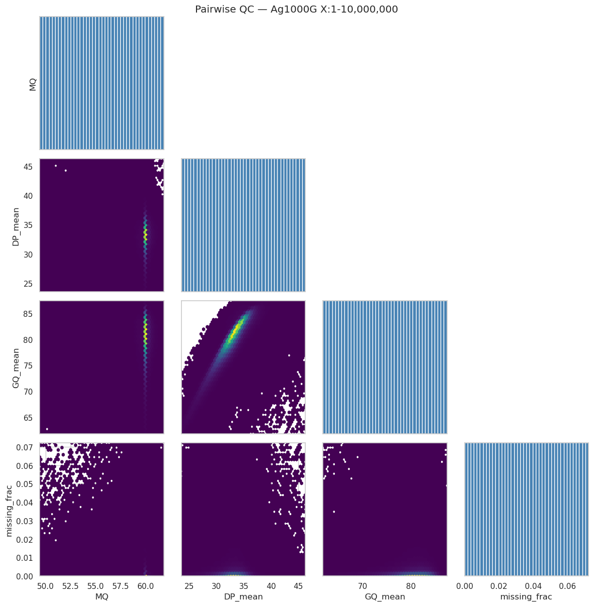
User prompt: $> Show me bivariate plots of all quality metrics against each other.
Skill action:
1. Drop columns flagged constant / all-NaN. 2. Render a lower-triangle hexbin matrix; diagonals are histograms. 3. Hexbin (not scatter) because there are ~10⁶ sites and scatter is unreadable past ~10⁴.
[4]:
import matplotlib.pyplot as plt
import seaborn as sns
sns.set_theme(context='notebook', style='whitegrid')


# Skill action: lower-triangle hexbin matrix (scatter is unreadable past ~1e4
# points; hexbin handles 1e5-1e6 cleanly). Diagonal = histogram of each
# column. Constant / all-NaN fields dropped before plotting.
def pairwise_hexbin(df, cols, gridsize=50, figsize=None, q_clip=(0.005, 0.995)):
    n = len(cols)
    figsize = figsize or (3.0 * n, 3.0 * n)
    fig, axes = plt.subplots(n, n, figsize=figsize, squeeze=False)
    lims = {}
    for c in cols:
        v = df[c].to_numpy().astype('f8')
        lo, hi = np.nanquantile(v, q_clip)
        if lo == hi:
            lo, hi = lo - 0.5, hi + 0.5
        lims[c] = (lo, hi)
    for i, ci in enumerate(cols):
        for j, cj in enumerate(cols):
            ax = axes[i, j]
            if i == j:
                v = df[ci].to_numpy().astype('f8')
                m = np.isfinite(v) & (v >= lims[ci][0]) & (v <= lims[ci][1])
                ax.hist(v[m], bins=40, color='steelblue')
                ax.set_yticks([])
            elif j < i:
                x = df[cj].to_numpy().astype('f8')
                y = df[ci].to_numpy().astype('f8')
                m = np.isfinite(x) & np.isfinite(y)
                ax.hexbin(x[m], y[m], gridsize=gridsize, mincnt=1, extent=(*lims[cj], *lims[ci]), cmap='viridis')
            else:
                ax.set_visible(False)
            if i == n - 1:
                ax.set_xlabel(cj)
            else:
                ax.set_xticks([])
            if j == 0:
                ax.set_ylabel(ci)
            else:
                ax.set_yticks([])
            ax.set_xlim(*lims[cj])
            ax.set_ylim(*lims[ci])
    fig.tight_layout()
    return fig

drop = flags.set_index('col')
drop = drop[drop['flag'].str.startswith(('ALL-NaN', 'constant'))].index.tolist()
biv_cols = [c for c in ['MQ', 'AN', 'AC_total', 'DP_mean', 'GQ_mean', 'missing_frac'] if c in site and c not in drop]
print(f'Plotting: {biv_cols}')
if drop:
    print(f'Dropped (constant / all-NaN): {drop}')
fig = pairwise_hexbin(site, biv_cols)
fig.suptitle('Pairwise QC — Ag1000G X:1-10,000,000', y=1.005)
plt.show()
Plotting: ['MQ', 'DP_mean', 'GQ_mean', 'missing_frac']
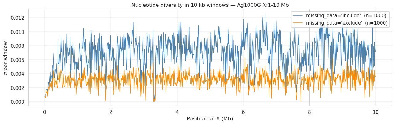
User prompt: $> Show me π calculated in 10,000 bp windows. What are my missingness options?
Skill action:
1. ``windowed_analysis(hm, window_size=10_000, step_size=10_000, statistics=[‘pi’], missing_data=mode)`` for each mode. 2. Two ``missing_data=`` modes are implemented:
'include'(default) — keep every site, use per-siten_validfor the SFS counts; unbiased under MCAR.*
'exclude'— drop sites with any missing call before computing. Stricter, but on cohorts with ~75% per-site missingness the surviving site count can be zero in entire windows.3. For most analyses'include'is the right default;'exclude'is a sanity check — if the two diverge, missingness is structured and needs upstream investigation.*
[5]:
from pg_gpu import windowed_analysis

hm = HaplotypeMatrix.from_zarr(ZARR_X, region='X:1-10000000', streaming='auto')
print(f'hm: {type(hm).__name__}  variants={hm.num_variants:,}  haps={hm.num_haplotypes:,}')

results = {}
for mode in ['include', 'exclude']:
    results[mode] = windowed_analysis(
        hm, window_size=10_000, step_size=10_000,
        statistics=['pi'], missing_data=mode,
    )
    print(f"{mode:9s}  windows={len(results[mode]):4d}   "
          f"median pi={results[mode]['pi'].median():.6f}   "
          f"mean pi={results[mode]['pi'].mean():.6f}")

fig, ax = plt.subplots(figsize=(13, 4.2))
colors = {'include': 'steelblue', 'exclude': 'darkorange'}
for mode, df in results.items():
    ax.plot(df['center'] / 1e6, df['pi'], lw=1.1, color=colors[mode],
            label=f"missing_data='{mode}'  (n={len(df)})")
ax.set_xlabel('Position on X (Mb)')
ax.set_ylabel(r'$\pi$ per window')
ax.set_title('Nucleotide diversity in 10 kb windows — Ag1000G X:1-10 Mb')
ax.legend(loc='upper right', frameon=True)
plt.tight_layout(); plt.show()
hm: HaplotypeMatrix  variants=7,610,313  haps=2,940
include    windows=1000   median pi=0.007287   mean pi=0.007035
exclude    windows=1000   median pi=0.003166   mean pi=0.003123
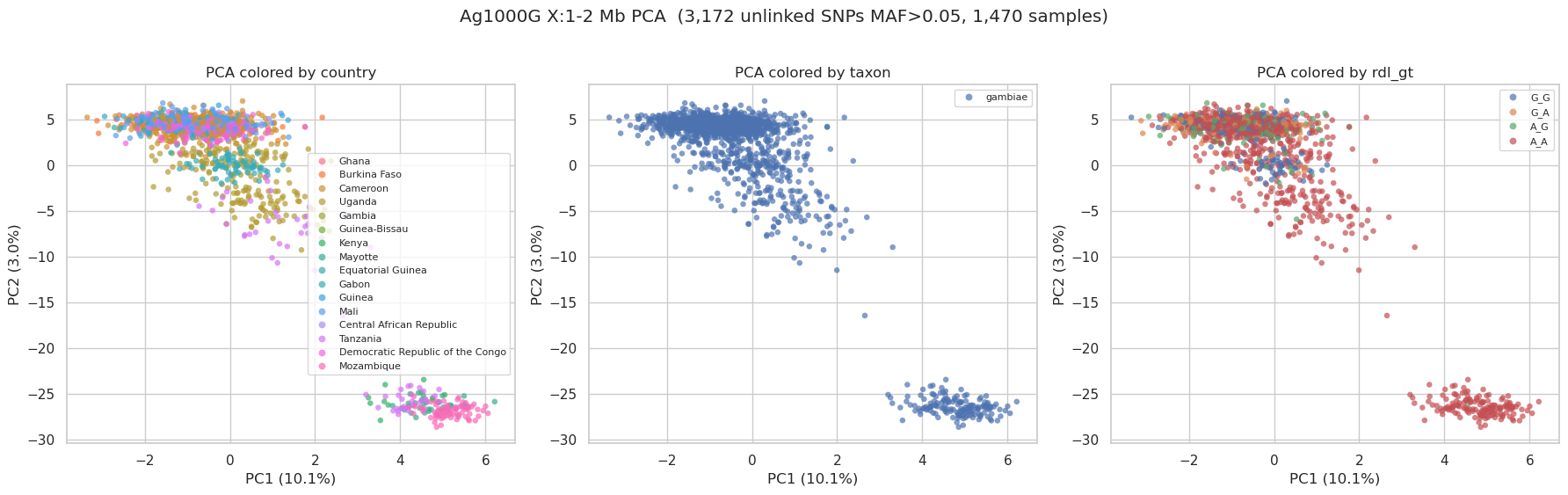
User prompt: $> Run a PCA and color the samples using the metadata file ag1000g_metadata.csv.
Skill action:
1. ``HaplotypeMatrix.from_zarr(region=’X:1-2000000’, streaming=’never’)`` then ``.apply_biallelic_filter()`` — PCA assumes 0/1 coding. 2. Filter sites with MAF > 0.05 — compute AF per site from ``hm.haplotypes`` (numpy), mask ``-1`` missing, drop monomorphic and rare. Subsumes ‘segregating only’. 3. ``hm.locate_unlinked(size=100, step=20, threshold=0.1)`` → ``get_subset()`` — LD-prune so PCs reflect population structure, not LD blocks. 4. ``decomposition.randomized_pca(hm, n_components=10)`` — faster than full SVD on big matrices. 5. Average per-haplotype coords to per-sample. pg_gpu’s VCZ-loaded matrix lays out the haplotype axis as ``[hap0 of every sample, then hap1 of every sample]`` — sample ``i``’s haplotypes are at rows ``i`` and ``i + n_samples``, NOT at ``2i`` and ``2i+1``. Average: ``(coords[:n_samples] + coords[n_samples:]) / 2``. 6. Merge with the metadata CSV on ``sample_id``, scatter PC1 vs PC2 colored by ``country``, ``taxon``, ``rdl_gt``.
[6]:
from pg_gpu import HaplotypeMatrix, decomposition
import zarr

META = 'ag1000g_metadata.csv'
meta = pd.read_csv(META)

z          = zarr.open(ZARR_X, mode='r')
sample_ids = list(z['sample_id'][:])
n_samples  = len(sample_ids)

# Load eagerly and biallelic-filter.
hm_raw = HaplotypeMatrix.from_zarr(ZARR_X, region='X:1-2000000', streaming='never')
hm_bi  = hm_raw.apply_biallelic_filter()
print(f'after biallelic filter: {hm_bi.num_variants:,} variants')

# MAF > 0.05. hm.haplotypes is a cupy array on a GPU-resident
# matrix; numpy ops below dispatch to cupy via NEP-18 so the math
# stays on the GPU. Convert with .get() only at the end.
haps    = hm_bi.haplotypes
n_valid = (haps >= 0).sum(axis=0)
alt     = (haps == 1).sum(axis=0)
af      = np.where(n_valid > 0, alt / np.maximum(n_valid, 1), 0.0)
maf     = np.minimum(af, 1.0 - af)
keep    = np.where(maf > 0.05)[0]
hm_common = hm_bi.get_subset(keep)
print(f'after MAF > 0.05:       {hm_common.num_variants:,} common variants')

# LD-prune.
unlinked = hm_common.locate_unlinked(size=100, step=20, threshold=0.1)
unlinked_np = unlinked.get() if hasattr(unlinked, 'get') else np.asarray(unlinked)
hm_pca   = hm_common.get_subset(np.where(unlinked_np)[0])
print(f'after LD prune:         {hm_pca.num_variants:,} unlinked SNPs')

# Randomized PCA.
coords, explained = decomposition.randomized_pca(hm_pca, n_components=10)
coords_np = coords.get() if hasattr(coords, 'get') else np.asarray(coords)
explained = explained.get() if hasattr(explained, 'get') else np.asarray(explained)

# pg_gpu layout: [hap0 of all samples, hap1 of all samples]
# Sample i's two haps are at rows i and i + n_samples.
coords_per_sample = (coords_np[:n_samples] + coords_np[n_samples:]) / 2.0

df = pd.DataFrame(coords_per_sample, columns=[f'PC{i+1}' for i in range(coords_per_sample.shape[1])])
df['sample_id'] = sample_ids
df = df.merge(meta, on='sample_id', how='left')
print(f'\nPC variance explained (top 5): '
      f'{[f"{v*100:.1f}%" for v in explained[:5]]}')

fig, axes = plt.subplots(1, 3, figsize=(18, 5.5))
for ax, hue in zip(axes, ['country', 'taxon', 'rdl_gt']):
    sns.scatterplot(data=df, x='PC1', y='PC2', hue=hue, ax=ax,
                    alpha=0.7, s=22, edgecolor='none')
    ax.set_xlabel(f'PC1 ({explained[0]*100:.1f}%)')
    ax.set_ylabel(f'PC2 ({explained[1]*100:.1f}%)')
    ax.set_title(f'PCA colored by {hue}')
    ax.legend(loc='best', fontsize=8, markerscale=1.2)
fig.suptitle(f'Ag1000G X:1-2 Mb PCA  ({hm_pca.num_variants:,} unlinked SNPs MAF>0.05, {n_samples:,} samples)', y=1.02)
plt.tight_layout(); plt.show()
after biallelic filter: 243,900 variants
after MAF > 0.05:       4,257 common variants
after LD prune:         3,172 unlinked SNPs

PC variance explained (top 5): ['10.1%', '3.0%', '1.1%', '0.5%', '0.4%']
User prompt: $> Set up populations from the metadata so the rest of the stats can compare groups.
Skill action:
1. Load a fresh 2 Mb biallelic matrix that the next several stat cells share: ``HaplotypeMatrix.from_zarr(region=’X:1-2000000’, streaming=’never’).apply_biallelic_filter()``. 2. Map ``country`` in the metadata to haplotype indices. pg_gpu lays the haplotype axis out as ``[hap0 of every sample, then hap1 of every sample]`` — sample ``i``’s haplotypes are at indices ``i`` and ``i + n_samples``, never consecutive pairs. 3. Keep the top 4 most-sampled countries. 4. Attach as ``hm_stats.sample_sets = {country: [hap_indices]}``.
[7]:
hm_stats = HaplotypeMatrix.from_zarr(ZARR_X, region='X:1-2000000', streaming='never')
hm_stats = hm_stats.apply_biallelic_filter()
print(f'hm_stats: {hm_stats.num_variants:,} biallelic variants x {hm_stats.num_haplotypes:,} haps')

n_samples = hm_stats.num_haplotypes // 2

# pg_gpu layout: hap-axis = [hap0 of all samples, hap1 of all samples].
# Sample i's haps are at indices i and i + n_samples, NOT 2i and 2i+1.
sample_to_idx = {s: i for i, s in enumerate(sample_ids)}
country_to_haps = {}
for country, gdf in meta.groupby('country'):
    haps = []
    for s in gdf['sample_id']:
        if s in sample_to_idx:
            i = sample_to_idx[s]
            haps.extend([i, i + n_samples])
    country_to_haps[country] = haps

top4 = sorted(country_to_haps, key=lambda k: -len(country_to_haps[k]))[:4]
hm_stats.sample_sets = {c: country_to_haps[c] for c in top4}
print('populations attached:')
for c, h in hm_stats.sample_sets.items():
    print(f'  {c:20s}  n_haps={len(h):,}  (n_diploids={len(h)//2})')
hm_stats: 243,900 biallelic variants x 2,940 haps
populations attached:
  Cameroon              n_haps=832  (n_diploids=416)
  Uganda                n_haps=414  (n_diploids=207)
  Burkina Faso          n_haps=314  (n_diploids=157)
  Mali                  n_haps=262  (n_diploids=131)
User prompt: $> Compute diversity stats (π, θ_W, Tajima’s D, expected heterozygosity) for each population in one shot.
Skill action:
1. For each population in ``hm_stats.sample_sets``, call ``diversity.diversity_stats(hm_stats, population=pop, statistics=[‘pi’,’theta_w’,’theta_h’,’theta_l’,’tajimas_d’])``. 2. Single GPU pass per population — much cheaper than calling each function separately. 3. Tabulate per-pop into a DataFrame.
[8]:
from pg_gpu import diversity

rows = []
for pop in hm_stats.sample_sets:
    s = diversity.diversity_stats(
        hm_stats, population=pop,
        statistics=['pi', 'theta_w', 'theta_h', 'theta_l', 'tajimas_d'],
    )
    # Convert any CuPy scalars to plain floats.
    s = {k: float(v.get() if hasattr(v, 'get') else v) for k, v in s.items()}
    s['n_diploids'] = len(hm_stats.sample_sets[pop]) // 2
    rows.append({'pop': pop, **s})

div_df = pd.DataFrame(rows).set_index('pop')
div_df.round(5)
[8]:
| pi | tajimas_d | theta_l | theta_h | theta_w | n_diploids | |
|---|---|---|---|---|---|---|
| pop | ||||||
| Cameroon | 0.00100 | -2.63267 | 0.00086 | 0.00071 | 0.00863 | 416 |
| Uganda | 0.00094 | -2.50651 | 0.00081 | 0.00069 | 0.00499 | 207 |
| Burkina Faso | 0.00101 | -2.61930 | 0.00085 | 0.00070 | 0.00608 | 157 |
| Mali | 0.00099 | -2.53713 | 0.00083 | 0.00068 | 0.00491 | 131 |
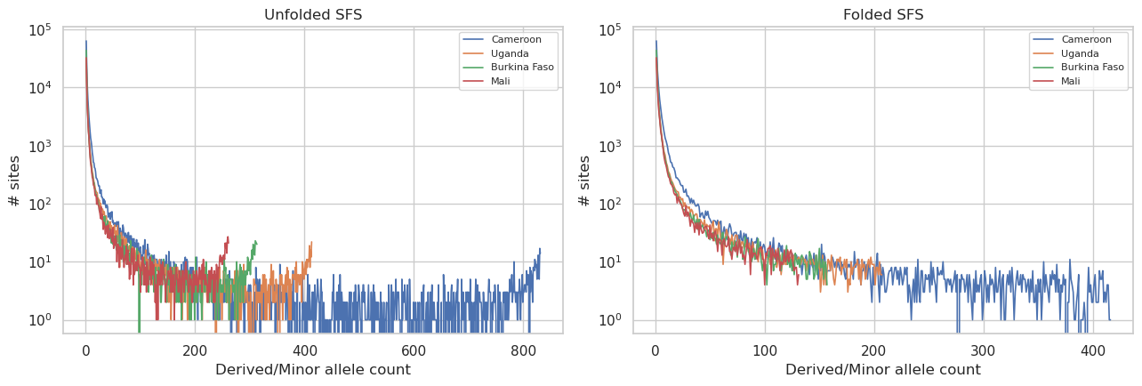
User prompt: $> Plot the unfolded and folded site frequency spectrum for each population side-by-side.
Skill action:
1. For each population: ``sfs.sfs(hm_stats, population=pop)`` for the unfolded spectrum, ``sfs.sfs_folded(hm_stats, population=pop)`` for the folded. 2. Each returns a length-``n_haps+1`` count vector. Drop the fixed bins (index 0 and index ``n_haps``) for readability. 3. Plot all populations on log-y axes — side-by-side panels.
[9]:
from pg_gpu import sfs as pg_sfs

fig, axes = plt.subplots(1, 2, figsize=(13, 4.5))
for pop in hm_stats.sample_sets:
    s_un = pg_sfs.sfs(hm_stats, population=pop)
    s_fo = pg_sfs.sfs_folded(hm_stats, population=pop)
    s_un = s_un.get() if hasattr(s_un, 'get') else np.asarray(s_un)
    s_fo = s_fo.get() if hasattr(s_fo, 'get') else np.asarray(s_fo)
    # Drop fixed bins (0 and n) for readability.
    axes[0].plot(np.arange(1, len(s_un)-1), s_un[1:-1], label=pop, lw=1.2)
    axes[1].plot(np.arange(1, len(s_fo)),   s_fo[1:],   label=pop, lw=1.2)
for ax, title in zip(axes, ['Unfolded SFS', 'Folded SFS']):
    ax.set_yscale('log'); ax.set_xlabel('Derived/Minor allele count')
    ax.set_ylabel('# sites'); ax.set_title(title); ax.legend(fontsize=8)
plt.tight_layout(); plt.show()
User prompt: $> Compute pairwise FST and dxy between every population pair.
Skill action:
1. For each ``(p1, p2)`` in ``itertools.combinations(pops, 2)``: ``divergence.fst(hm_stats, p1, p2)`` (Hudson FST by default) and ``divergence.dxy(hm_stats, p1, p2)``. 2. Tabulate into a long-form DataFrame, pivot to a symmetric matrix. 3. Render as two heatmaps side-by-side.
[10]:
from pg_gpu import divergence
from itertools import combinations

pops = list(hm_stats.sample_sets)
rows = []
for p1, p2 in combinations(pops, 2):
    fst = divergence.fst(hm_stats, p1, p2)
    dxy = divergence.dxy(hm_stats, p1, p2)
    rows.append({'pop1': p1, 'pop2': p2,
                 'fst':  float(fst.get() if hasattr(fst, 'get') else fst),
                 'dxy':  float(dxy.get() if hasattr(dxy, 'get') else dxy)})
pairwise = pd.DataFrame(rows)

# Build symmetric matrices for a quick visual.
fst_mat = pairwise.pivot(index='pop1', columns='pop2', values='fst').reindex(index=pops, columns=pops)
fst_mat = fst_mat.fillna(0) + fst_mat.fillna(0).T
dxy_mat = pairwise.pivot(index='pop1', columns='pop2', values='dxy').reindex(index=pops, columns=pops)
dxy_mat = dxy_mat.fillna(0) + dxy_mat.fillna(0).T

fig, axes = plt.subplots(1, 2, figsize=(11, 4.5))
sns.heatmap(fst_mat, annot=True, fmt='.4f', cmap='viridis', ax=axes[0],
            cbar_kws={'label': 'FST'})
sns.heatmap(dxy_mat, annot=True, fmt='.4f', cmap='viridis', ax=axes[1],
            cbar_kws={'label': 'dxy'})
axes[0].set_title('Pairwise Hudson FST'); axes[1].set_title('Pairwise dxy')
plt.tight_layout(); plt.show()
pairwise.round(5)
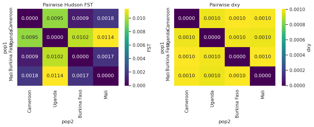
[10]:
| pop1 | pop2 | fst | dxy | |
|---|---|---|---|---|
| 0 | Cameroon | Uganda | 0.00955 | 0.00098 |
| 1 | Cameroon | Burkina Faso | 0.00088 | 0.00101 |
| 2 | Cameroon | Mali | 0.00179 | 0.00100 |
| 3 | Uganda | Burkina Faso | 0.01024 | 0.00098 |
| 4 | Uganda | Mali | 0.01139 | 0.00098 |
| 5 | Burkina Faso | Mali | 0.00168 | 0.00100 |
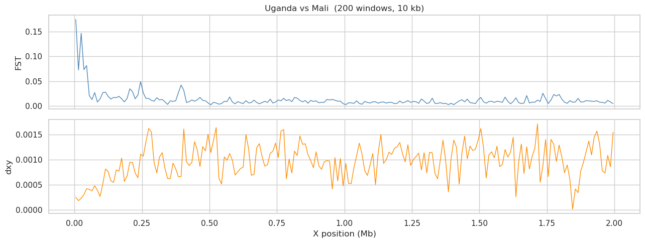
User prompt: $> Run windowed FST and dxy across the 2 Mb region for one population pair.
Skill action:
1. Pick the most-diverged pair from the previous heatmap (highest FST). 2. Single GPU pass: ``windowed_analysis(hm_stats, window_size=10_000, step_size=10_000, statistics=[‘fst’,’dxy’], populations=[p1, p2], missing_data=’include’)``. 3. Plot FST and dxy across the region in two stacked panels sharing the X axis.
[11]:
from pg_gpu import windowed_analysis

# Most diverged pair (max FST) from the previous step.
p1, p2 = pairwise.sort_values('fst', ascending=False).iloc[0][['pop1', 'pop2']]
print(f'windowed FST/dxy: {p1} vs {p2}')

wdf = windowed_analysis(
    hm_stats, window_size=10_000, step_size=10_000,
    statistics=['fst', 'dxy'],
    populations=[p1, p2],
    missing_data='include',
)
fst_col = next(c for c in wdf.columns if c.startswith('fst'))
dxy_col = next(c for c in wdf.columns if c.startswith('dxy'))

fig, axes = plt.subplots(2, 1, figsize=(13, 5), sharex=True)
axes[0].plot(wdf['center']/1e6, wdf[fst_col], lw=1, color='steelblue')
axes[0].set_ylabel('FST'); axes[0].set_title(f'{p1} vs {p2}  ({len(wdf)} windows, 10 kb)')
axes[1].plot(wdf['center']/1e6, wdf[dxy_col], lw=1, color='darkorange')
axes[1].set_ylabel('dxy'); axes[1].set_xlabel('X position (Mb)')
plt.tight_layout(); plt.show()
windowed FST/dxy: Uganda vs Mali
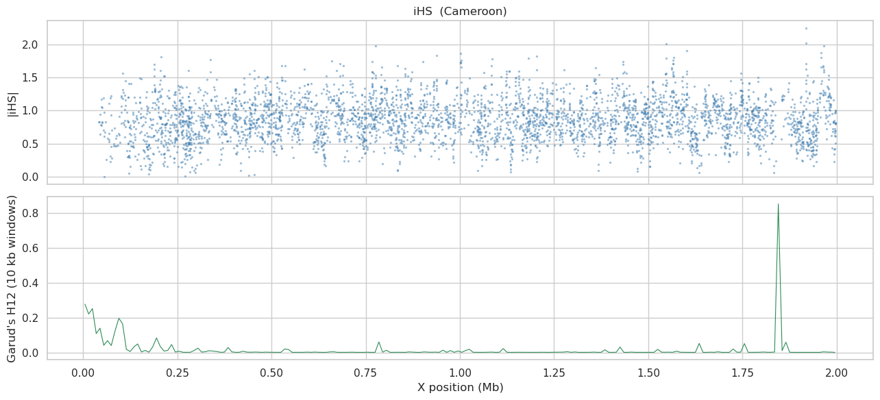
User prompt: $> Run a selection scan (iHS + Garud’s H) on the largest population.
Skill action:
1. iHS and Garud’s H are single-population statistics; pass ``population=pop`` per population, otherwise the scan mixes all four into one (rarely informative). 2. ``selection.ihs(hm_stats, population=pop)`` returns per-site iHS scores (shape ``(n_variants,)``); ``selection.garud_h(…)`` returns four scalars ``(h1, h12, h123, h2_h1)`` — for a position-vs-statistic curve use ``windowed_analysis(statistics=[‘garud_h12’], populations=[pop])``. 3. pg_gpu does not inspect or enforce phase — it treats every VCF ``GT`` as two haplotypes regardless of ``/`` vs ``|``. iHS / Garud are only meaningful when the input is statistically phased upstream (Ag1000G Ag3.0 is SHAPEIT-phased, so the assumption holds). 4. Plot |iHS| (per-site) and H12 (per-window) for the largest population.
[12]:
from pg_gpu import selection

biggest = max(hm_stats.sample_sets, key=lambda k: len(hm_stats.sample_sets[k]))
print(f'selection scans (per-pop) for plotting: {biggest} '
      f'(n_haps={len(hm_stats.sample_sets[biggest])})')

# Per-population iHS (per-site scores).
ihs_arr = selection.ihs(hm_stats, population=biggest)
ihs = ihs_arr.get() if hasattr(ihs_arr, 'get') else np.asarray(ihs_arr)

# Per-population windowed Garud's H12 (selection.garud_h returns SCALARS;
# for a position-vs-statistic plot use the windowed variant instead).
h12_df = windowed_analysis(
    hm_stats, window_size=10_000, step_size=10_000,
    statistics=['garud_h12'], populations=[biggest],
)
h12_col = next(c for c in h12_df.columns if c.startswith('garud_h12'))

pos = hm_stats.positions
if hasattr(pos, 'get'): pos = pos.get()

fig, axes = plt.subplots(2, 1, figsize=(13, 6), sharex=True)
valid = np.isfinite(ihs)
axes[0].scatter(pos[valid]/1e6, np.abs(ihs[valid]), s=2, alpha=0.4, color='steelblue')
axes[0].set_ylabel('|iHS|'); axes[0].set_title(f'iHS  ({biggest})')

axes[1].plot(h12_df['center']/1e6, h12_df[h12_col], lw=0.8, color='seagreen')
axes[1].set_ylabel("Garud's H12 (10 kb windows)"); axes[1].set_xlabel('X position (Mb)')
plt.tight_layout(); plt.show()
selection scans (per-pop) for plotting: Cameroon (n_haps=832)
User prompt: $> Compute the proper 2-locus LD statistics (D², Dz, π_2) binned by bp distance — the moments-LD curves used for demographic inference.
Skill action:
1. moments-LD is O(n_var²) per pop per pair per bin. Restrict to a smaller region and two populations so this finishes in minutes, not hours. 2. Load fresh 500 kb biallelic: ``HaplotypeMatrix.from_zarr(region=’X:1-500000’, streaming=’never’).apply_biallelic_filter()``. Reuse the top-2 populations from ``hm_stats.sample_sets``. 3. ``from pg_gpu.moments_ld import compute_ld_statistics; compute_ld_statistics(haplotype_matrix=hm_ld, pop_assignment=…, pops=…, bp_bins=np.logspace(2,5,10).astype(int), ac_filter=True)``. 4. Output structure: ``ld_stats[‘stats’] = [ld_names, het_names]``; ``ld_stats[‘sums’] = [bin1_LD, bin2_LD, …, het_sums]`` — last entry has a different shape (the het summary). 5. Filter ``sums`` to LD-shaped arrays only, stack to ``(n_bins, n_ld_stats)``, plot the within-population curves ``DD_i_i``, ``Dz_i_i_i``, ``pi2_i_i_i_i``.
[13]:
from pg_gpu import moments_ld, ld_statistics

# moments-LD is O(n_var^2) per pop / per pair / per bin -- on the full
# 2 Mb biallelic matrix (~240k variants) it takes ~20 min even with two
# populations. For a demo that finishes in minutes, drop to a fresh
# 500 kb biallelic load and the top-two populations.
hm_ld = (HaplotypeMatrix
         .from_zarr(ZARR_X, region='X:1-500000', streaming='never')
         .apply_biallelic_filter())
ld_pops = list(hm_stats.sample_sets)[:2]
hm_ld.sample_sets = {p: hm_stats.sample_sets[p] for p in ld_pops}
print(f'hm_ld: {hm_ld.num_variants:,} biallelic variants  /  pops: {ld_pops}')

bp_bins = np.logspace(2, 5, 10).astype(int)
ld_stats = moments_ld.compute_ld_statistics(
    haplotype_matrix=hm_ld,
    pop_assignment={p: hm_ld.sample_sets[p] for p in ld_pops},
    pops=ld_pops,
    bp_bins=bp_bins,
    ac_filter=True,
    report=False,
)

# moments-LD output structure:
#   ld_stats['stats'] = [ld_names, het_names]    (two lists)
#   ld_stats['sums']  = [bin1_ld, bin2_ld, ..., binN_ld, het_sums]
#     The first N entries are per-bp-bin LD stats (shape == len(ld_names));
#     the last entry is the het summary (shape == len(het_names)).
ld_names  = list(ld_stats['stats'][0])
het_names = list(ld_stats['stats'][1])
n_ld      = len(ld_names)

ld_arrays = [np.asarray(a) for a in ld_stats['sums']
             if np.asarray(a).ndim == 1 and len(np.asarray(a)) == n_ld]
sums_per_bin = np.stack(ld_arrays)                                    # (n_bins, n_ld)
print(f'output: {sums_per_bin.shape[0]} LD-stat bins x {sums_per_bin.shape[1]} stats')
print(f'  first 6 stat names: {ld_names[:6]}')

bin_centers = np.sqrt(bp_bins[:-1] * bp_bins[1:])
sums_per_bin = sums_per_bin[: len(bin_centers)]

def curve(stat_name):
    if stat_name not in ld_names:
        return None
    return sums_per_bin[:, ld_names.index(stat_name)]

# Plot within-population D², Dz, pi2 for each population. Suffix _i_j(_k_l)
# convention: DD_i_i = within-pop i; Dz_i_i_i and pi2_i_i_i_i likewise.
fig, axes = plt.subplots(1, 3, figsize=(15, 4.2), sharex=True)
stat_specs = [
    ('DD',  [f'DD_{i}_{i}'           for i in range(len(ld_pops))]),
    ('Dz',  [f'Dz_{i}_{i}_{i}'       for i in range(len(ld_pops))]),
    ('pi2', [f'pi2_{i}_{i}_{i}_{i}'  for i in range(len(ld_pops))]),
]
for ax, (title, keys) in zip(axes, stat_specs):
    plotted = False
    for i, k in enumerate(keys):
        y = curve(k)
        if y is None:
            continue
        ax.plot(bin_centers, y, marker='o', lw=1.0, label=ld_pops[i])
        plotted = True
    if not plotted:
        ax.text(0.5, 0.5, f'no {title} stats matched', ha='center', va='center',
                transform=ax.transAxes); ax.set_xticks([]); ax.set_yticks([])
        continue
    ax.set_xscale('log'); ax.set_xlabel('Pair separation (bp)')
    ylab = r'$\langle \pi_2 \rangle$' if title == 'pi2' else fr'$\langle {title} \rangle$'
    ax.set_title(title); ax.set_ylabel(ylab); ax.legend(fontsize=8)
plt.tight_layout(); plt.show()

# Reference scalar for context, computed on the full 2 Mb matrix.
zns = ld_statistics.zns(hm_stats)
zns = float(zns.get() if hasattr(zns, 'get') else zns)
print(f'\nReference: ZnS (mean pairwise r^2 over the 2 Mb hm_stats) = {zns:.4f}')
hm_ld: 58,416 biallelic variants  /  pops: ['Cameroon', 'Uganda']
output: 9 LD-stat bins x 15 stats
  first 6 stat names: ['DD_0_0', 'DD_0_1', 'DD_1_1', 'Dz_0_0_0', 'Dz_0_0_1', 'Dz_0_1_1']
Reference: ZnS (mean pairwise r^2 over the 2 Mb hm_stats) = 0.0000
User prompt: $> Give me a block-jackknife confidence interval on π for the largest population.
Skill action:
1. ``resampling.block_jackknife`` operates on pre-binned per-block values — it does not take a HaplotypeMatrix and has no ``block_size=`` kwarg. 2. First compute per-block π in non-overlapping windows of the block size you want: ``windowed_analysis(hm_stats, window_size=200_000, step_size=200_000, statistics=[‘pi’], populations=[pop])``. 3. Extract the per-window π array, pass through ``resampling.block_jackknife(pi_per_block, statistic=lambda v: np.mean(v))`` → ``(estimate, se, _)``. 4. Approximate normal-theory 95% CI: ``estimate ± 1.96 × se``. 5. 200 kb is reasonable for taxa with ~kb-scale LD decay; tune from the LD-decay panel above.
[14]:
from pg_gpu import resampling

biggest = max(hm_stats.sample_sets, key=lambda k: len(hm_stats.sample_sets[k]))

# Per-block pi at 200 kb resolution.
df_blocks = windowed_analysis(
    hm_stats, window_size=200_000, step_size=200_000,
    statistics=['pi'], populations=[biggest],
)
pi_col = next(c for c in df_blocks.columns if c.startswith('pi'))
pi_per_block = df_blocks[pi_col].to_numpy()
print(f'{len(pi_per_block)} blocks of 200 kb for population {biggest!r}')

pi_est, pi_se, _ = resampling.block_jackknife(
    pi_per_block,
    statistic=lambda v: float(np.mean(v)),
)
pi_est = float(pi_est); pi_se = float(pi_se)
ci_lo, ci_hi = pi_est - 1.96 * pi_se, pi_est + 1.96 * pi_se

print(f'pi ({biggest}):  estimate = {pi_est:.6f}')
print(f'               SE        = {pi_se:.6f}')
print(f'               95% CI    = [{ci_lo:.6f}, {ci_hi:.6f}]')
10 blocks of 200 kb for population 'Cameroon'
pi (Cameroon):  estimate = 0.001000
               SE        = 0.000056
               95% CI    = [0.000891, 0.001109]
[ ]: